Examples
Arrivals Time and Calendars
For this example we used the log that we can find in the folder example_arrivals/BPIChallenge2012A.xes. This event log pertains to a loan application process of a Dutch financial institute. The data contains all applications filed trough an online system in 2016 and their subsequent events until February 1st 2017, 15:11. The company providing the data and the process under consideration is the same as doi:10.4121/uuid:3926db30-f712-4394-aebc-75976070e91f.
The petrinet found by the inductive miner is the following:

In this example we want to show different ways to generate the arrivals times of tokens in the simulation. As exaplained in the inter_trigger_timer class we can define the arrivals with 3 methods:
- Distribution function: specify in the json file the distribution with the right parameters in seconds, see the numpy_distribution.
    "interTriggerTimer": {
        "type": "distribution",
        "name": "exponential",
        "parameters": {
            "scale": 300
        }
    }
In addition, it is possible to add a schedule for token arrival times, i.e. when a new instance of the process can start. For example, we establish that a new trace of this process can start only from Monday to Friday, from 8 a.m. to 3 p.m.
    "interTriggerTimer": {
        "type": "distribution",
        "name": "exponential",
        "parameters": {
            "scale": 20
        },
        "calendar": {
            "days": [0, 1, 2, 3, 4],
            "hour_min": 8,
            "hour_max": 15
        }
    }
To set a fixed time interval between arrivals, simply define a uniform distribution with the min and max parameters of the same value. As in the following example where we set 5 minutes (i.e. 300 seconds) between each token.
    "interTriggerTimer": {
        "type": "distribution",
        "name": "uniform",
        "parameters": {
            "low": 300,
            "high": 300
        }
    }
- Custom method: it is possible to define a dedicated method to define the next arrival (CUSTOM).
    "interTriggerTimer": {
        "type": "custom"
    }
In the following example we define a simple time series model from the python library (statsmodels). The AutoReg model is trained on the real log and then we used it to predict the next token arrival in the process.
Finally, we defined the two calendars for Role 1 and Role 2 with the following code. Role 1 resources, Sara and Mike, work Monday through Friday, 8 a.m. to 4 p.m.
   "Role 1": {
        "resources": ["Sara", "Mike"],
        "calendar": {
            "days": [0, 1, 2, 3, 4],
            "hour_min": 8,
            "hour_max": 16
        }
   }
While Role 2 resources, Ellen and Sue, work Monday through Saturday, 8 a.m. to 7 p.m.
   "Role 2": {
        "resources": ["Ellen", "Sue"],
        "calendar": {
            "days": [0, 1, 2, 3, 4, 5],
            "hour_min": 8,
            "hour_max": 19
        }
   }
To run the example with a exponential distribution:
python run_simulation.py -p example/example_arrivals/bpi2012.pnml -s /example/example_arrivals/input_arrivals_example_distribution.json -t 20 -i 1 -o example_arrivals
or use the short command
python run_simulation.py -e arrivalsD
To run the example with a time series model:
python run_simulation.py -p example/example_arrivals/bpi2012.pnml -s example/example_arrivals/input_arrivals_example_timeseries.json -t 10 -i 1 -o example_arrivals
or use the short command
python run_simulation.py -e arrivalsS
Decision Mining of petrinet
For this example we used the log that we can find in the folder example_decision_mining/BPIChallenge2012A.xes. This event log pertains to a loan application process of a Dutch financial institute. The data contains all applications filed trough an online system in 2016 and their subsequent events until February 1st 2017, 15:11. The company providing the data and the process under consideration is the same as doi:10.4121/uuid:3926db30-f712-4394-aebc-75976070e91f. Every process execution represents a single application to the bank by a customer for a personal loan. The application can be accepted or rejected by the bank, likewise the customer can withdraw the application at any time.
The petrinet found by the Inductive Miner algorithm from pm4py, is the following:

We also want to show how to add a case-specific attribute, requested loan amount, to each simulation trace. Through the function case_function_attribute(case_id) it is easy to add the attribute/s case with the return of a dictionary. In this case, for each trace, we randomly generate a loan amount from 1000 to 99999 euros.
    def case_function_attribute(case):
        return {"AMOUNT": random.randint(1000, 99999)}
The aim of this example is to present different ways to choose the next activity from a specific decision point of Petri net model. In the following image, the four decision points in the process are highlighted with three different colours.
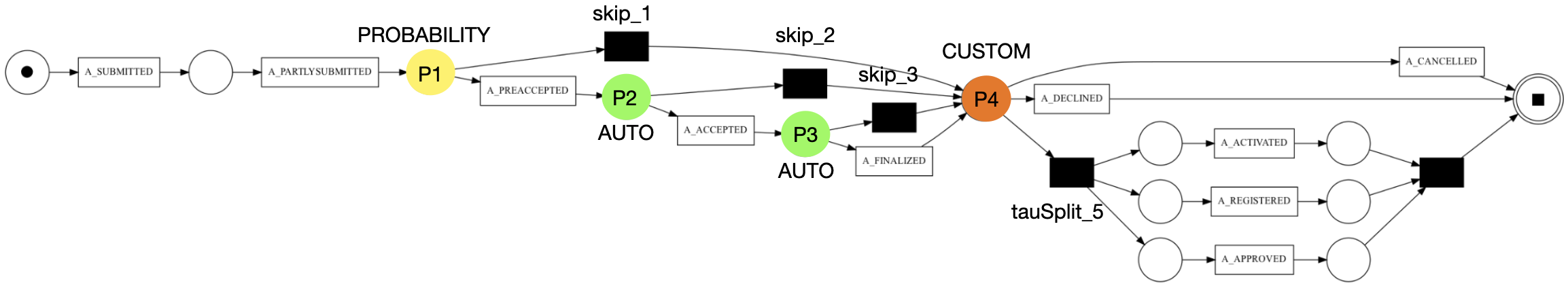
As exaplained in the event trace class, we can define the 3 methods to define the next activity of decision point:
- Random choice: each path has equal probability to be chosen for green points (AUTO).
    "probability": {
        "skip_2": "AUTO",
        "A_ACCEPTED": "AUTO",
        "skip_3": "AUTO",
        "A_FINALIZED": "AUTO"
    }
- Defined probability: in the file json it is possible to define for each path a specific probability, in this case for the yellow point. (PROBABILITY as value)
    "probability": {
        "A_PREACCEPTED": 0.20,
        "skip_1": 0.80
    }
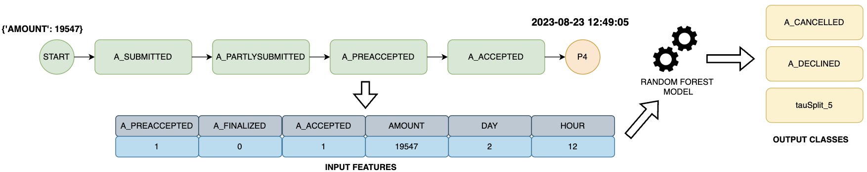
- Custom method: it is possible to define a dedicate method that given the possible paths it returns the one to
follow, using whatever techniques the user prefers. In this case for the orange point we trained a
simple Random Forest to predict the next activity. (CUSTOM)
   "probability": {
      "A_CANCELLED": "CUSTOM",
      "A_DECLINED": "CUSTOM",
      "tauSplit_5": "CUSTOM"
   }
To train the model we used as input the following feature: the presence of A_PREACCEPTED, A_ACCEPTED, A_FINALIZED activities in the prefix of trace, the requested loan amount, the weekday and hour of the time of arrival in the decision point.
In general, if the user does not define probability parameters in the JSON file, the simulator automatically applies the AUTO mode for each decision point. Otherwise, if the user defines the mode for one or more decision points, the user still has to specify all of them even if they are in AUTO mode.
To run the example:
python main.py -p ../example/example_decision_mining/bpi2012.pnml -s ../example/example_decision_mining/input_decision_mining_example.json -t 10 -i 1 -o example_decision_mining
or use the short command
python run_simulation.py -e decision_mining
Process Times of petrinet
For this example, we used the log located in the example_process_times/synthetic_log.xes folder. To generate the synthetic log we define a simulation model inspired by the BPIC2012 process (the log in the other two examples). The log contains 4000 traces with 20 different activities.
Let's define the following Petri net model to generate a new simulation.

The aim of this example is to present several ways to set the processing time of each activity and the waiting time between them.
As explained in custom_function, we can apply two methods to define processing and waiting times:
Distribution function: specify in the json file the distribution with the right parameters for each activity, see the numpy_distribution.
"A_FINALIZED": {
    "name": "uniform",
    "parameters": {
        "low": 3600,
        "high": 7200
    }
}
- Custom method: a dedicated method can be defined that, given the activity and its features, returns the processing time duration or the needed waiting time. (CUSTOM)
  "processing_time": {
      "A_FINALIZED":  { "name": "custom"}
  }
Be careful: The simulator raises a WARNING if the distribution produces a negative value as processing/waiting time and instead sets the value to zero.
For this example, two random forests are trained to predict the processing time of the activity W_Complete_preaccepted_appl and the waiting time before the activity W_Call_after_offer. The remaining processing times are set with different probability distributions, and the waiting times are undefined, except for the A_REGISTERED activity. For the latter, it is assumed that 5 to 10 minutes are required to prepare documentation for registration, which is not included in the processing time. Therefore, the waiting times between the remaining activities are generated only by resource contention.
"waiting_time": {
    "W_Call_after_offer": {
       "name": "custom"
    },
    "A_REGISTERED": {
        "name": "uniform",
        "parameters": {
            "low": 300,
            "high": 600
        }
    }
}
The following figure describes the features involved in training the two random forest models. All features except "start_time" are intercase features that RIMS can provide during simulation. From the code shown, it can be seen that it is simple to predict the prediction at runtime using the intercase features.
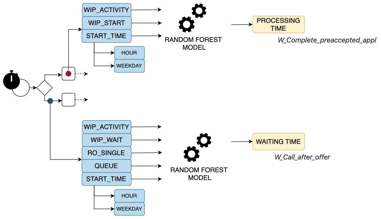
- To predict the processing time of the activity W_Complete_preaccepted_appl with the following features.
def custom_processing_time(buffer: Buffer):
    input_feature = list()
    input_feature.append(buffer.get_feature("wip_start"))
    input_feature.append(buffer.get_feature("wip_activity"))
    input_feature.append(buffer.get_feature("start_time").weekday())
    input_feature.append(buffer.get_feature("start_time").hour)
    loaded_model = pickle.load(open(os.getcwd()+'/example/example_process_times/processing_time_random_forest.pkl', 'rb'))
    y_pred_f = loaded_model.predict([input_feature])
    return int(y_pred_f[0])
- To predict the waiting time before the activity W_Call_after_offer
def custom_waiting_time(buffer: Buffer):
    input_feature = list()
    buffer.print_values()
    input_feature.append(buffer.get_feature("wip_wait"))
    input_feature.append(buffer.get_feature("wip_activity"))
    input_feature.append(buffer.get_feature("enabled_time").weekday())
    input_feature.append(buffer.get_feature("enabled_time").hour)
    input_feature.append(buffer.get_feature("ro_single"))
    input_feature.append(buffer.get_feature("queue"))
    loaded_model = pickle.load(
        open(os.getcwd() + '/example/example_process_times/waiting_time_random_forest.pkl', 'rb'))
    y_pred_f = loaded_model.predict([input_feature])
    return int(y_pred_f[0])
To run the example:
python main.py -p ../example/example_decision_mining/bpi2012.pnml -s ../example/example_decision_mining/input_decision_mining_example.json -t 10 -i 1 -o example_decision_mining
or use the short command
python run_simulation.py -e process_times
To see more complex case studies, it is possible to refer to the following papers: Runtime integration of machine learning and simulation for business processes (to appear at the ICPM conference) and Recommending the optimal policy by learning to act from temporal data. In the second paper, an ad-hoc version of ${RIMS}{\mathsf{_{Tool}}}$ is used to simulate the behavior of the environment in response to agent action recommended by the optimal policy discovered in a Reinforcement Learning scenario.
 1"""
 2.. include:: ../README.md
 3.. include:: example/example_arrivals/arrivals-example.md
 4.. include:: example/example_decision_mining/decision_mining-example.md
 5.. include:: example/example_process_times/process_times-example.md
 6"""
 7
 8import csv
 9import simpy
10import utility
11from process import SimulationProcess
12from event_trace import Token
13from parameters import Parameters
14import sys, getopt
15from utility import *
16import pm4py
17from inter_trigger_timer import InterTriggerTimer
18from result_analysis import Result
19from datetime import timedelta
20import warnings
21import sys
22
23EXAMPLE = {'arrivalsD': ['example/example_arrivals/bpi2012.pnml', 'example/example_arrivals/input_arrivals_example_distribution.json', 1, 15, 'example_arrivals'],
24           'arrivalsS': ['example/example_arrivals/bpi2012.pnml', 'example/example_arrivals/input_arrivals_example_timeseries.json', 1, 15, 'example_arrivals'],
25           'process_times': ['example/example_process_times/synthetic_petrinet.pnml', 'example/example_process_times/input_process_times_example.json', 1, 15, 'example_process_times'],
26           'decision mining': ['example/example_decision_mining/bpi2012.pnml', 'example/example_decision_mining/input_decision_mining_example.json', 1, 10, 'example_decision_mining'],
27           }
28
29
30def setup(env: simpy.Environment, PATH_PETRINET, params, i, NAME):
31    simulation_process = SimulationProcess(env, params)
32    utility.define_folder_output("output/output_{}".format(NAME))
33    f = open("output/output_{}/simulated_log_{}_{}".format(NAME, NAME, i)+".csv", 'w')
34    writer = csv.writer(f)
35    writer.writerow(Buffer(writer).get_buffer_keys())
36    net, im, fm = pm4py.read_pnml(PATH_PETRINET)
37    interval = InterTriggerTimer(params, simulation_process, params.START_SIMULATION)
38    for i in range(0, params.TRACES):
39        prefix = Prefix()
40        itime = interval.get_next_arrival(env, i)
41        yield env.timeout(itime)
42        parallel_object = utility.ParallelObject()
43        time_trace = params.START_SIMULATION + timedelta(seconds=env.now)
44        env.process(Token(i, net, im, params, simulation_process, prefix, 'sequential', writer, parallel_object, time_trace, None).simulation(env))
45
46
47def run_simulation(PATH_PETRINET, PATH_PARAMETERS, N_SIMULATION, N_TRACES, NAME):
48    params = Parameters(PATH_PARAMETERS, N_TRACES)
49    for i in range(0, N_SIMULATION):
50        env = simpy.Environment()
51        env.process(setup(env, PATH_PETRINET, params, i, NAME))
52        env.run(until=params.SIM_TIME)
53
54    result = Result("output_{}".format(NAME), params)
55    result._analyse()
56
57
58def main(argv):
59    opts, args = getopt.getopt(argv, "h:p:s:t:i:o:e:")
60    for opt, arg in opts:
61        print(opt, arg)
62        if opt == '-h':
63            print('main.py -p <petrinet in pnml format> -s <parameters read from file .json> -t <total number of traces> -i <total number of simulation>')
64            sys.exit()
65        elif opt == "-p":
66            PATH_PETRINET = arg
67        elif opt == "-s":
68            PATH_PARAMETERS = arg
69        elif opt == "-t":
70            N_TRACES = int(arg)
71        elif opt == "-i":
72            N_SIMULATION = int(arg)
73        elif opt == "-o":
74            NAME = arg
75        elif opt == "-e":
76            if arg in EXAMPLE:
77                PATH_PETRINET, PATH_PARAMETERS, N_SIMULATION, N_TRACES, NAME = EXAMPLE[arg]
78            else:
79                raise ValueError('The keywords for the provided examples are the following: arrivalsD, arrivalsS, decision_mining, process_times')
80    print(PATH_PETRINET, PATH_PARAMETERS, N_SIMULATION, N_TRACES, NAME)
81    run_simulation(PATH_PETRINET, PATH_PARAMETERS, N_SIMULATION, N_TRACES, NAME)
82
83
84if __name__ == "__main__":
85    warnings.filterwarnings("ignore")
86    main(sys.argv[1:])